Finding Limits Algebraically: Determinate and Indeterminate Forms
By the end of this lecture, you should be able to recognize which undefined expressions are determinate and which are indeterminate, and you should be able to use this knowledge to solve limit problems by rewriting them algebraically until you obtain a determinate form. In particular, you should be able to find limits at infinity, and to determine when the limits do not exist (and when they do not exist, to explain why). You should also be able to use limit notation correctly.
Before we begin this lecture, we want to remind ourselves about an algebra definition that will be important when calculating limit problems algebraically:
Definition: undefined
Remember that in algebra we sometimes get expressions that are undefined. An undefined expression is one that doesn't have one clear value - for example, if we could prove that an expression has two different values, then that expression would be undefined because we don't allow expressions to be equal to two different things at once (because this would lead to crazy contradictions like 2=5!).
Another reason an expression might be undefined, is because it is undefined with respect to the set of numbers we are currently working with. For example, if we are only working in the set of real numbers, any expression which gives us an imaginary or complex number as our answer will be undefined in the set of real numbers. We don't always say very explicitly which set of numbers we are working under, but for the duration of this class, we will only be looking at real numbers (notice that on our graphs, there is no way to graph an imaginary or complex number).
For example, you should have encountered problems like these in a previous algebra class
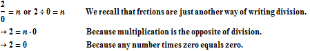
2/0 is undefined, because there is no good way for us to define this mathematically without leading to a contradiction. For example, let's suppose this value is defined and that it is actually equal to some number, which we decide to call n. Then by definition, we would have:
But this is a contradiction! Two is NOT equal to zero!
In fact, we notice that there is NO value that we could put in for n in the equation above that would make this equation true, because no matter what value we try to use for n, the statement 2 = n·0 will NEVER be true.
So there is no way we can make sense of a number that has zero as its denominator, because there is no way can define a single value to be equal to that number.
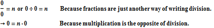
0/0 is undefined, because, like 2/0,there is no good way for us to define this mathematically without leading to a contradiction. For example, let's suppose this value is defined and that it is actually equal to some number, which we decide to call n. Then by definition, we would have:
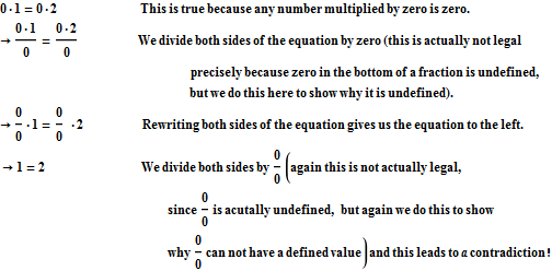
This seems OK at first, because whatever value we put in for n will make the equation true. However, that is precisely the problem: ANY value we put in for n will make the equation true, so 0/0 could be defined to be many different UNEQUAL possible values. In other words, it can't be assigned only one value, without also assigning it other unequal values. To see why this is true, let's look at a simple equation:
But this is a contradiction! One is NOT equal to two!
So there is no way we can make sense of a number that has zero as its denominator, even if it also has zero in the numerator.
In this case, is undefined over the set of real numbers whenever n is negative, because it will produce an imaginary number in this case. Because cannot be equal to any REAL number when n is negative, it is undefined over the set of real numbers (but not over the set of complex numbers, which includes imaginary numbers).
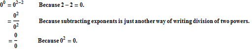
This is an example of an undefined expression that you may not have seen before. However, we can quickly see that it is undefined because it can be rewritten as the expression 0/0, which we already know is undefined:
Because 0/0 is undefined, 00 must also be undefined, since we have just shown that these two expressions are equivalent.
(Actually, sometimes mathematicians decide to treat 00 as equal to 1, even though it's not clear that this is true - it's more of a convention. To read an interesting discussion of how and why this is done, take a look at this webpage!)
When we calculate limit problems algebraically, we will often obtain as an initial answer something that is undefined. This is because the "interesting" places to look for limits are places where a function is undefined. Because the function f(x) is undefined at x=c, f(c) will produce an expression that is undefined. However, it is important for us to remember that when we are calculating the limit of f(x) as x→c we are not interested in the behavior of f(x) AT c, but rather the behavior of f(x) AROUND c. So, this leads us to the motivating question for this lecture:
When we get an undefined value at f(c), can the type of undefined value that we get tell us something about the behavior of f(x) AROUND x=c?
We'll spend the rest of this lecture playing around with limit problem examples in an attempt to answer this question!
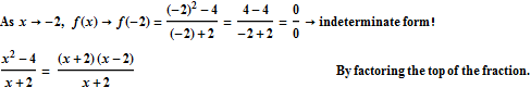
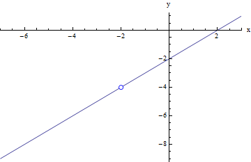
Let's begin by recalling Example #2 from the last lecture:
The graph of f(x) was a line with a hole in it at x = -2:
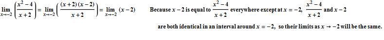
In this case when we replaced f(x) with x -2, what we were actually doing was replacing f(x), which is a line with a hole at x = -2, with y = x -2, which is the exact same line without the hole. The two functions are not completely identical, but they identical everywhere except at x = -2, which is all that matters when we are calculating the limit. In order for two functions to have the same limit at x = -2, all we need is for them to be identical in some interval aroundx = -2 (but NOT necessarily atx = -2).
So, let's summarize the steps we encountered when doing these problems:
We tried calculating f(c) directly, but found that it was undefined (in this case because it was equal to 0/0).
We found a way to replace f(x) with a different function that is the same as f(x) everywhere except at x=c (in this case by factoring the top and the bottom of the fraction and canceling out a common factor).
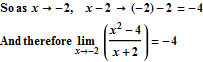
We calculated the limit of that new function by substituting in c for x, and this time we got a value that was not undefined. Because the new function is the same as the f(x) everywhere except at x=c, the limits of the two functions are the same, so we can conclude that the limit of f(x) is the same.
We will see that this same pattern occurs in many of the limit problems that we will tackle. The one main difference will be that sometimes the type of undefined value that we get will tell us something about what the behavior is of f(x) in the interval around x=c, and sometimes the indeterminate form will not provide us enough information about what happens to f(x) around x=c, and in that case we will need to perform more algebra steps, as we did above, to rewrite f(x) so that plugging in c for x will give us specific information about the behavior of f(x) around x=c.
Let's look at some examples.
But just before we dive into the examples, let's take a moment to clarify some notation:
Notation: The use of 0 and ∞ when calculating limits.
In the last lecture we saw how we may calculate f(c) as one step towards trying to determine what the limit of f(x) is as x approaches c. In cases where f(c) exists, this is simple, because then the limit will be equal to f(c). However, in most cases we are calculating the limit precisely because f(c) does NOT exist, and in those cases, calculating f(c) will always produce an undefined expression. In these cases, when we compute f(c), what we are actually doing is thinking about what f(c+) and f(c-) are.
In other words, we need to remember that when we are trying to evaluate a limit by substituting in c for x, we are NOT actually plugging in the value c exactly, but rather we are substituting in values that are arbitrarily CLOSE to c but NOT actually EQUAL to c.
Zero:
For example, if we say that as x→c, what we really mean is that f(x) is a fraction for which the top and bottom both get arbitrarily close to zero as x gets closer and closer to c. However, neither the top nor the bottom of the fraction ever actually reach zero. In other words, both the top and the bottom of f(x) are shrinking in magnitude as x gets closer and closer to c. So, the zeros in the expression INSERT are NOT really zeros - rather, they are standing in for numbers that have very small magnitudes (i.e. are very very close to zero).
Infinity:
Similarly, when we use the notation ∞ when calculating limits, we don't actually mean infinity. Remember that what we mean by ±∞ is really just a pattern of unbounded behavior where the magnitude of the numbers grows ever larger, without bound.
So, for example, if I find that as x→ -∞, then what this really means is that f(x) is an expression for which the first and second terms both get arbitrarily large in magnitude as x gets arbitrarily more and more negative. However, neither the first nor the second term of the expression ever actually reach infinity, because that is not possible. Infinity is not a number that can be reached. In other words, both the first and second term in f(x) are growing unbounded in magnitude as x gets more and more negative. So, the infinity signs in the expression INSERT NOTATIONEX2.GIF HERE are NOT really infinities - rather, they are standing in for numbers that have very large magnitudes (i.e. are very very far away from zero).
When evaluating limit expressions, both 0 and ∞ are standing in for a type of BEHAVIOR AROUND x=c:
0 stands for some number that is arbitrarily close to zero;
+∞ stands for some number that is arbitrarily large; and
-∞ stands for some number that is negative but has an arbitrarily large magnitude.
Now let's move on to those examples!
Calculating Limits Algebraically: Examples
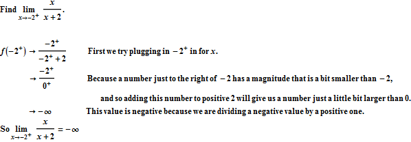
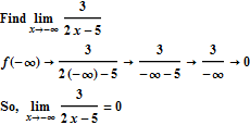
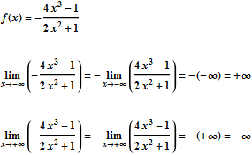
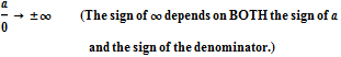
Example 1: When f(c) yields the undefined expression a/0, where a≠0
In this example, when we calculate f(c), we will initially get an expression of the form a/0 where a≠0 (i.e. a fraction where the top number is some fixed non-zero value but the bottom number is zero):
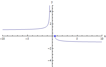
In this case, f(x) → -∞ as x → -2 from the right because f(x) approaches as x approaches -2 from the right. In other words, as x approaches -2 from the right, the numerator of f(x) becomes very close to -2 while the denominator's magnitude grows ever smaller. If we divide numbers that are arbitrarily close to -2 by positive numbers with increasingly smaller magnitude, we get negative numbers with increasingly larger magnitude as a result. And if put numbers in the denominator with a small enough magnitude, we can get numbers with as large a magnitude as we want - so this behavior is unbounded. As a result, we can say that f(x) will decrease without bound as x approaches -2 from the right, and we can write that f(x) → -∞ as x → -2.
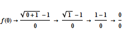
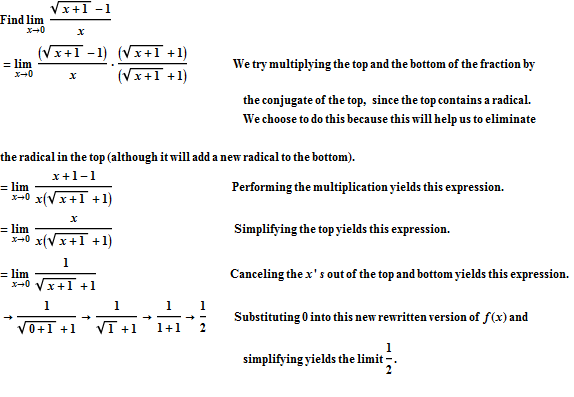
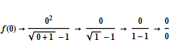
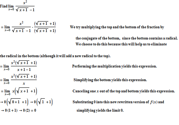
Example 2: When f(c) yields the undefined expression 0/0, but the actual limit of f(x) as x approaches c is a specific finite non-zero number
In this example, when we calculate f(c), we will initially get an expression of the form 0/0, but after using algebra to replace f(x) with a similar expression that is the same around (but NOT AT) x=c, we will be able to calculate the actual limit. This limit will turn out to be a specific finite number that is not zero in this case.
In this case, f(x) approaches 0/0 as x approaches 0. In other words, as x approaches 0, the magnitudes of both the numerator and the denominator of f(x) grow ever smaller. This is not enough information for us to conclude anything about the limit, because dividing numbers with increasingly smaller magnitude by other numbers with increasingly smaller magnitude can produce a number of different results: it depends on how "small" the magnitude of the numerator is in comparison to the denominator! And we don't know anything about the relationship between the numerator and the denominator yet.
So in this case, we need to look for a way to replace f(x) with a similar function that will be the same as f(x) all AROUND x=c, but not necessarily AT x=c. For this, we ask ourselves if there is any algebra that we could use to rewrite f(x) without changing its value anywhere other than at x=c . In this case, because f(x) contains a radical in the numerator, one possible approach is for us to try to rewrite the expression so that the radical in the numerator is canceled out - this may then allow us to cancel something out of the top and bottom of the fraction. (We won't be able to get rid of the radical entirely, and still keep the function the same around x=c, but we can move it, for example from the numerator to the denominator.)
Before moving on to more examples that will help us to better understand what can happen when we get the indeterminate form 0/0 for f(c), let's take a moment to note how we approached the solution to this problem, which will be the same underlying approach for ALL the examples in this lecture (and for calculating limits algebraically in general):
Big Idea: Algebra is just a way of Looking for Structure.
We often need expressions, equations, or other mathematical objects to have a SPECIFIC STRUCTURE in order for us to apply a particular rule or use a particular technique on them.
For example, you may recall that in a prior algebra class, when you wanted to solve a quadratic equation, you needed it to be in the form ax2 + bx + c = 0, so that you could factor the expression on the left-hand side of the equation, and then set each factor equal to zero (because if several things multiply together to get zero, you can conclude that at least one of those factors must be zero). If you encountered a quadratic equation which was not in this form (like 4 - x2 = -4x, for example), you would need to perform algebraic operations on the equation so that you could replace the original equation with an equivalent equation that has the form that you want. In this case, two equations are equivalent if they have the same solution set (the same values of x that make the equation true). So, for example, if I wanted to put 4 - x2 = -4x into the form ax2 + bx + c = 0, I can rearrange the terms in the equation so that it looks like this: 1x2 + -4x + -4 = 0. This equation has exactly the same solutions as the original equation 4 - x2 = -4x, but it is written in the form we want (because in this new form, it is easy to factor and then solve).
Right now we are interested in finding limits, and the only way we know how to find limits so far is to simply plug in c for x, and to calculate f(c). But sometimes this doesn't work - sometimes just plugging in c for x gives us something that is not defined, like . So in those cases, we want to ask ourselves, "What underlying structure in this expression is causing it to come out as undefined when I plug in c for x, and is there a way for me to replace it with another expression that is the same everywhere around x=c, but which will not produce an undefined result when we plug in c for x?".
So, in future, whenever we get an indeterminate form for f(c), the first thing that we will ask ourselves is, "How can we rewrite f(x) to get something that is equivalent (at least aroundx=c), but which has a different structure that will help us to avoid that particular indeterminate form?
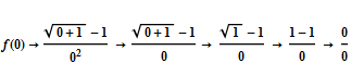
Example 3: When f(c) yields the undefined expression 0/0, but the actual limit of f(x) as x approaches c is zero
In this example, when we calculate f(c), we will initially get an expression of the form 0/0, but after using algebra to replace f(x) with a similar expression that is the same around (but NOT AT) x=c, we will be able to calculate the actual limit. This limit will turn out to be zero in this case.
Just as in the last example, f(x) approaches 0/0 as x approaches 0. Again, as x approaches 0, the magnitudes of both the numerator and the denominator of f(x) grow ever smaller, and this is not enough information for us to conclude anything about the limit, because it depends on how "small" the magnitude of the numerator is in comparison to the denominator, and therefore depends on the relationship between the numerator and the denominator.
So just as in the last example, in this case we need to look for a way to replace f(x) with a similar function that will be the same as f(x) all AROUND x=c, but not necessarily AT x=c. Again we ask ourselves if there is any algebra that we could use to rewrite f(x) without changing its value anywhere other than at x=c . In this case, because f(x) contains a radical in the denominator, one possible approach is for us to try to rewrite the expression so that the radical in the denominator is canceled out - this may then allow us to cancel something out of the top and bottom of the fraction. (Again, as in the last example, we won't be able to get rid of the radical entirely, and still keep the function the same around x=c, but we can move it, for example from the denominator to the numerator.)
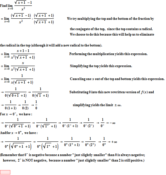
Example 4: When f(c) yields the undefined expression 0/0, but f(x) → ± ∞ as x approaches c
In this example, when we calculate f(c), we will initially get an expression of the form 0/0, but after using algebra to replace f(x) with a similar expression that is the same around (but NOT AT) x=c, we will be able to calculate the actual limit. In this case the limit will not exist because f(x) will decrease without bound as x approaches 0 from the left, and increase without bound as x approaches 0 from the right.
Just as in the last two examples, f(x) approaches 0/0 as x approaches 0. Again, as x approaches 0, the magnitudes of both the numerator and the denominator of f(x) grow ever smaller, and this is not enough information for us to conclude anything about the limit, because it depends on how "small" the magnitude of the numerator is in comparison to the denominator, and therefore depends on the relationship between the numerator and the denominator.
So just as in the last two examples, in this case we need to look for a way to replace f(x) with a similar function that will be the same as f(x) all AROUND x=c, but not necessarily AT x=c. Again we ask ourselves if there is any algebra that we could use to rewrite f(x) without changing its value anywhere other than at x=c . In this case, because f(x) contains a radical in the numerator, one possible approach is for us to try to rewrite the expression so that the radical in the numerator is canceled out - this may then allow us to cancel something out of the top and bottom of the fraction. (Again, as in the last example, we won't be able to get rid of the radical entirely, and still keep the function the same around x=c, but we can move it, for example from the numerator to the denominator.)
This problem is similar to example 1 above. In this case, f(x) → -∞ as x → 0 from the left because f(x) approaches as x approaches 0 from the left. In other words, as x approaches 0 from the left, the numerator of f(x) becomes very close to 1 while the denominator's magnitude grows ever smaller, and dividing a relatively fixed positive number (like 1) by negative numbers with increasingly smaller magnitude, we get negative numbers with increasingly larger magnitude as a result. And as in example 1, this behavior is unbounded (because by making the magnitude of the denominator small enough, we can get numbers with as big a magnitude as we want). So we can say that f(x) will decrease without bound as x approaches 0 from the left, and we can write that f(x) → -∞ as x → 0-. Similarly, f(x) →∞ as x → 0 from the right because f(x) approaches as x approaches 0 from the right.
What is the difference between examples 1, 2, 3 and 4?
Let's think back about these four examples, and summarize the differences between these four somewhat similar problems. In each of these examples f(x) was a fraction that had a zero in the denominator when we substituted c in for x, but in each case, the numerator and denominator of f(x) had different relationships as x got closer and closer to c:
In example 1, as x got ever closer to c, the numerator of f(x) approached a fixed number, while the magnitude of the denominator shrank indefinitely. This resulted in numbers with a magnitude that increased without bound (because dividing a relatively fixed value with numbers that are ever closer to zero results in numbers with an increasingly large magnitude, and because by making the magnitude of the denominator small enough, we can get numbers with as big a magnitude as we want).
In example 2, 3, and 4, as x got ever closer to c, the magnitudes of both the numerator and the denominator of f(x) shrank indefinitely. However:
In example 2, the magnitude of the numerator and the denominator shrank at roughly "the same" rate, so that when dividing the numerator by the denominator we get a fixed value that is very close to 1/2. (In this case, it is not really possible for us to see that they will "shrink at roughly the same rate" directly; we are only able to determine this by first rewriting the function using algebra.)
In example 3, the magnitude of the numerator shrank much more quickly than the magnitude of the denominator, so that when dividing the numerator by the denominator we get values that are ever-closer to zero. (In this case, it can be difficult to see that the magnitude of the numerator will shrink "much more quickly", but again, we are able to determine that this is the case by rewriting the function using algebra.)
In example 4, the magnitude of the denominator shrank much more quickly than the magnitude of the numerator, so that when dividing the numerator by the denominator we get values that have an ever-larger unbounded magnitude. (In this case, it can be difficult to see that the magnitude of the denominator will shrink "much more quickly", but again, we are able to determine that this is the case by rewriting the function using algebra.)
So what is the larger pattern here?
The four examples we just looked at showed us that:
When f(c) = a/0 for some a≠0, then this is enough information to tell us that f(x)→ ± ∞ as x → c, because dividing a relatively fixed value with numbers that are ever closer to zero results in numbers with an increasingly large magnitude, and because by making the magnitude of the denominator small enough, we can get numbers with as big a magnitude as we want.
When f(c) = 0/0, then this is NOT enough information to tell us anything about what happens to f(x) as x → c, because it does not tell us anything about the relationship between the numerator and the denominator. We know that the magnitudes of both the numerator and the denominator are shrinking indefinitely, but we don't know if they are shrinking at about the same rate (and therefore the ratio of the numerator to the denominator is remaining relatively fixed), or if the magnitude of one of them is shrinking "much faster" than the other (and therefore the ratio of the numerator to the denominator is either shrinking towards zero or increasing/decreasing without bound).
In this case, we must use algebra to replace f(x) with a similar function (that is the same as f(x) AROUND but not necessarily AT x=c) that does NOT give us 0/0 when we plug in c for x.
We note that BOTH a/0 (when a≠0) and 0/0 are undefined, but that a/0 tells us something about the limit behavior (even though it is undefined), while 0/0 doesn't give us any useful information about the limit behavior.
So whenever we get an undefined value for f(c), we will need to stop and ask ourselves whether the undefined form that we get tells us anything about the limit behavior of f(x) AROUND x=c or not. This leads us to a few definitions that we will use to describe this distinction:
Definition: Indeterminate and Determinate Forms
When we are looking for limx →cf(x) and plugging c in for x produces an undefined expression for f(c):
That undefined expression is determinate if it gives us enough information to determine what the limit behavior is of f(x) AROUND x=c, without having to do further calculations. (e.g. a/0 for a≠0)
That undefined expression is indeterminate if there is more than one possible type of limit behavior of f(x) AROUND x=c which could produce that particular undefined expression. In other words, the indeterminate form doesn't give us enough information to determine what the behavior is of f(x) AROUND x=c, and so we will have to do further calculations to figure this out. (e.g. 0/0)
Careful! Notice that these definitions only have meaning when we are calculating a limit. If I am simply doing an algebra problem and I get a/0 or 0/0 as an answer, my final answer to that problem would simply be that the problem is undefined. It would be incorrect in that context for me to say anything about determinate or indeterminate forms, because I am not calculating a limit!
Now let's return to some more examples that give us other undefined expressions when we calculate f(c), and let's see if we can determine which undefined values for f(c) are indeterminate versus determinate forms!
Example 5: When f(c) yields the undefined expression b/±∞
In this example, when we calculate f(c), we will initially get an expression of the form b/±∞ (i.e. a fraction where the top number is some fixed value but the bottom is infinity):
In this case, f(x) → 0 as x → -∞ because f(x) approaches as the magnitude of x grows without bound. In other words, as x decreases without bound (i.e. becomes more and more negative), the numerator of f(x) becomes very close to 3 while the denominator's magnitude grows ever larger. If we divide numbers that are arbitrarily close to 3 by negative numbers with increasingly larger magnitude, we get negative numbers with increasingly smaller magnitude as a result. So we get numbers that are closer and closer to zero. As a result, we can write that f(x) → 0 as x → -∞.
Example 6: When f(c) yields the undefined expression±∞/b
In this example, when we calculate f(c), we will initially get an expression of the form ±∞/b (i.e. a fraction where the bottom number is some fixed value but the top is infinity):
In this case, f(x) → +∞ as x → +∞ because f(x) approaches as the magnitude of x grows without bound. In other words, as x increases without bound, the denominator of f(x) becomes very close to 0 while the numerator's magnitude grows ever larger. If we divide positive numbers that have an increasingly larger magnitude by positive numbers with an increasingly smaller magnitude (i.e. that are close to zero), we get positive numbers with increasingly larger magnitude as a result. As a result, we can write that f(x) → +∞ as x → +∞.
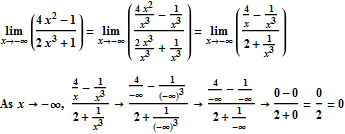
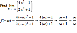
Example 7: When f(c) yields the undefined expression ±∞/±∞, but the actual limit of f(x) as x approaches c is zero
In this example, when we calculate f(c), we will initially get an expression of the form ±∞/±∞, but after using algebra to replace f(x) with a similar expression that is the same as x → -∞, we will be able to calculate the actual limit. This limit will turn out to be zero in this case.
In this case, f(x) approaches ∞/-∞ as x approaches -∞. In other words, as the magnitude of x grows without bound, the magnitudes of both the numerator and the denominator of f(x) grow ever larger. This is not enough information for us to conclude anything about the limit, because dividing numbers with increasingly larger magnitude by other numbers with increasingly larger magnitude can produce a number of different results: it depends on how "large" the magnitude of the numerator is in comparison to the denominator! And we don't know anything about the relationship between the numerator and the denominator yet.
So in this case, we need to look for a way to replace f(x) with a similar function that will be the same as f(x)as x → -∞ (but not necessarily everywhere else). For this, we ask ourselves if there is any algebra that we could use to rewrite f(x) without changing its value for negative x-values with particularly large magnitude. In this case, the problem is essentially that there are x's in both the numerator and the denominator: this means that whenever we plug in -∞ for x, we will inevitably end up with an infinity sign in both the numerator and the denominator. So we need to think of something that we can do to "rewrite" f(x) so that we can get rid of the x's in either the numerator or the denominator. This would change the form we get when we calculate f(c) from the indeterminate form ±∞/±∞ to a determinate form that is either b/±∞ or ±∞/b, and we know that and that .
So, in order to do that, we begin by noticing that the largest power of x in the numerator is x2: So, if we were to divide everything in the numerator and the denominator by x2, we would be able to "cancel out" the powers of x in the numerator, with the aim of keeping the numerator from tending towards infinity when we plug in -∞ for x:
There is also more than one way to solve this problem. The method used above is just one example, but the limit can also be found in a different way, using a similar algebraic technique, but this time dividing by the largest power of x overall, instead of just the largest power of x in the numerator. Notice that either method works equally well in helping us to find the limit, giving us the same answers in both cases:
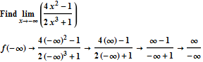
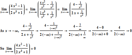
Example 8: When f(c) yields the undefined expression ±∞/±∞, but the actual limit of f(x) as x approaches c is a fixed non-zero number
In this example, when we calculate f(c), just like in the last example we will initially get an expression of the form ±∞/±∞, but this time after using algebra to replace f(x) with a similar expression that is the same as x → -∞, we will be able to calculate the actual limit. This limit will turn out to be 2.
Similarly to the last example, f(x) approaches ∞/∞ as x approaches -∞. Just as before, as the magnitude of x grows without bound, the magnitudes of both the numerator and the denominator of f(x) grow ever larger, and once again this is not enough information for us to conclude anything about the limit, because we don't know anything about the relationship between the numerator and the denominator yet.
So just as in the last problem, we need to look for a way to replace f(x) with a similar function that will be the same as f(x) as x → -∞, and again we notice that the largest power of x in the numerator is x2: So, just as in the last example, if we were to divide everything in the numerator and the denominator by x2, we would be able to "cancel out" the powers of x in the numerator, with the aim of keeping the numerator from tending towards infinity when we plug in -∞ for x:
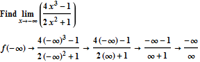
Example 9: When f(c) yields the undefined expression ±∞/±∞, but f(x) → ± ∞ as x approaches c
In this example, when we calculate f(c), just like in the last two examples we will initially get an expression of the form ±∞/±∞, but this time after using algebra to replace f(x) with a similar expression that is the same as x → -∞, we will find that f(x) →-∞ as x → -∞.
Similarly to the last example, f(x) approaches -∞/∞ as x approaches -∞. Just as before, as the magnitude of x grows without bound, the magnitudes of both the numerator and the denominator of f(x) grow ever larger, and once again this is not enough information for us to conclude anything about the limit, because we don't know anything about the relationship between the numerator and the denominator yet.
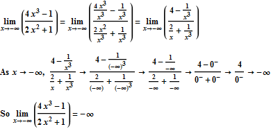
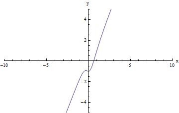
So just as in the last two problems, we need to look for a way to replace f(x) with a similar function that will be the same as f(x) as x → -∞, and again using the same sort of approach as in these problems, we notice that the largest power of x in the numerator is x3: So, just as in the last example, if we were to divide everything in the numerator and the denominator by x3, we would be able to "cancel out" the powers of x in the numerator, with the aim of keeping the numerator from tending towards (negative) infinity when we plug in -∞ for x:
What is the larger pattern in this case?
The five examples we just looked at showed us that:
When f(c) = b/±∞, then this is enough information to tell us that f(x)→ 0 as x → c, because dividing a relatively fixed value with numbers of increasing magnitude results in numbers which are ever-closer to zero.
When f(c) = ±∞/b, then this is enough information to tell us that f(x)→ ±∞ as x → c, because dividing a value with ever-increasing magnitude with a value that remains relatively fixed, results in numbers with larger and larger magnitude, and we can obtain a number of any magnitude as the result by making the magnitude of the numerator large enough.
When f(c) = ±∞/±∞, then this is NOT enough information to tell us anything about what happens to f(x) as x → c, because it does not tell us anything about the relationship between the numerator and the denominator. We know that the magnitudes of both the numerator and the denominator are growing without bound, but we don't know if they are growing at about the same rate (and therefore the ratio of the numerator to the denominator is remaining relatively fixed), or if the magnitude of one of them is growing "much faster" than the other (and therefore the ratio of the numerator to the denominator is either shrinking towards zero or increasing/decreasing without bound).
In this case, we must use algebra to replace f(x) with a similar function (that is the same as f(x) AROUND but not necessarily AT x=c) that does NOT give us ±∞/±∞ when we plug in c for x.
So far we've looked at two categories of determinant and indeterminate forms:
a/0, where a≠0, is a determinate form which tends towards ±∞, while 0/0 is an indeterminate form.
b/±∞ is a determinate form which tends toward 0; ±∞/b is a determinant form which tends towards ±∞; and ±∞/±∞ is an indeterminate form.
But these aren't the only two examples of formats that produce determinant and indeterminate forms. There are a number of other determinant and indeterminate forms which we will encounter when working on trying to solve limit problems algebraically. Here is a table which shows all of the determinant and indeterminate forms:
Reference Table: Indeterminate and Determinate Forms
Determinant and Indeterminate Forms Here ∞ = +∞, a, b, and c are arbitrary fixed real numbers, a≠0, c≠1, and c>0.
Indeterminate Forms
Determinant Forms
Careful! We note that when an expression has a ± symbol in more than one place, the ± does not necessarily mean the same thing in both places! For example, if we have a·±∞ → ±∞, the ± sign to the left of the arrow and the ± to the right of the arrow may not have the same sign: if a is negative, they will have opposite signs, for example.
So any time we calculate f(c) by plugging in c for x, when our goal is really to find the limit of f(x) as x approaches c, we know that if the result is on the list of indeterminate forms above, we will need to do more work before we can calculate the limit (usually by rearranging f(x) using some algebra). However, if the expression we get for f(c) is on the list of determinant forms, we already know what the limit of f(x) will be as x approaches c.
But we don't want to simply use this list blindly! If we simply look up values on this list, without really understanding why the expressions on the left are indeterminate while the expressions on the right are determinant, we are likely to make a mistake at some point and apply these ideas incorrectly. Furthermore, it's much easier for us to understand why each of these forms is determinant or indeterminate than it is to simply memorize the list without understanding it. It's easy to forget a list of expressions that we have memorized, but it is much harder to forget an idea that we actually understand. So, I strongly recommend that you make sure that you understand how to explain in your own words why each of these forms is either indeterminate or determinant (and if it is determinant, what the value of the limit will be).
We've already looked at examples and discussed how we classified the first two lines of the table as determinant or indeterminate, so now let's explore some of the other expressions:
What is the difference between ∞ - ∞ and ∞+∞?
In the third row of our table we notice that ∞ - ∞ (or -∞+∞) is indeterminate, while ∞+∞ (or -∞ - ∞) is determinant - why is this the case? Let's think about this and then work out some limit examples. We can see that ∞+∞ must tend toward ∞ because adding two values together, both of which are increasing without bound, will just give us a third value that is also increasing without bound. (Similarly -∞ - ∞ will give us something that is decreasing without bound.)
However, if we think about ∞ - ∞, we can see that we run into the problem that we don't know the relationship between the first and the second value:
It could be that the magnitude of the first value is increasing "much faster" than the second value, in which case ∞ - ∞ would tend toward +∞.
It could be that the magnitude of the second value is increasing "must faster" than the first value, in which case ∞ - ∞ would tend toward -∞.
Or, it could be that magnitudes of both the first and the second values are increasing at "about the same" rate, in which case ∞ - ∞ would tend toward 0 or some other fixed value.
So, until we know more about the relationship between the first and the second value in the expression ∞ - ∞, we don't know what to conclude about the limit behavior of f(x) around x=c.
This one is also easy to think about graphically: We can think of the expression ∞ - ∞ as describing two graphs (one graph for the first term and one for the second term), each of which are increasing without bound, and then ∞ - ∞ stands for the distance between the two graphs as x approaches c. If the first and the second graph are two parallel lines with a positive slope, each line will grow without bound as x→∞, but the distance between the two lines will remain fixed as x→∞. However, if one of those lines is steeper than the other, the distance between the two lines will grow as x→∞.
Let's look at some worked out examples for these different cases of the determinant form ∞+∞ (or -∞ - ∞) and the indeterminate form ∞ - ∞:
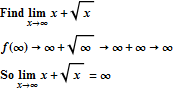
Example 10: When f(c) yields the undefined expression ∞+∞, so f(x) → ∞ as x approaches c
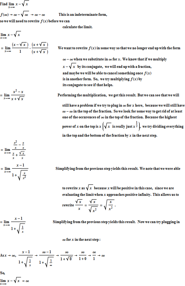
Example 11: When f(c) yields the undefined expression ∞ - ∞, but f(x) → ∞ as x approaches c
We notice that in this case, the magnitude of the first term grows "more quickly" than the magnitude of the second term.
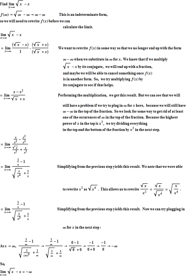
Example 12: When f(c) yields the undefined expression ∞ - ∞, but f(x) → -∞ as x approaches c
We notice that in this case, the magnitude of the second term grows "more quickly" than the magnitude of the first term.
Example 13: When f(c) yields the undefined expression ∞ - ∞, but f(x) approaches zero as x approaches c
We notice that in this case, the magnitudes of both the first and second terms grow at about "the same" rate.
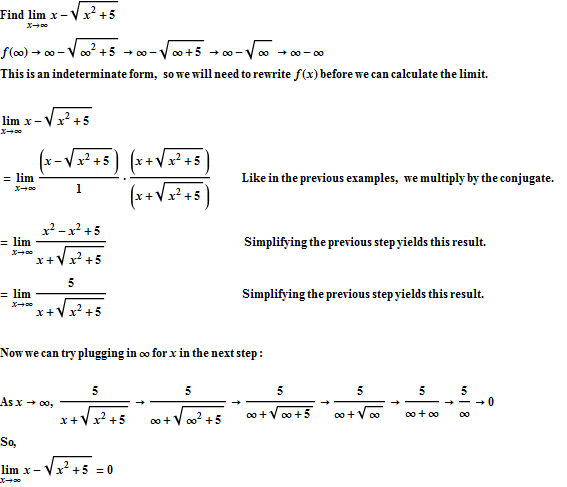
Example 14: When f(c) yields the undefined expression ∞ - ∞, but f(x) approaches a fixed finite non-zero value as x approaches c
We notice that in this case, the magnitudes of both the first and second terms grow at about "the same" rate.
Now that we've explored the determinant form ∞+∞ (or -∞ - ∞) and the indeterminate form ∞ - ∞, let's take a look at the different cases of the determinant forms a·±∞ and ±∞·±∞, and the indeterminate form 0·±∞:
What is the difference between 0·±∞ and the two cases a·±∞ and ±∞·±∞?
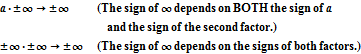
In the fourth row of our table we notice that 0·±∞ is indeterminate, while a·±∞ and ±∞·±∞ are determinant - why is this the case? We can see that a·±∞ and ±∞·±∞ must tend toward ±∞ because multiplying two values together, both of which have magnitudes that are increasing without bound, will just give us a third value whose magnitude is also increasing without bound (although its sign will depend on the signs of the two factors being multiplied together).
However, if we think about 0·±∞, we can see that we run into the problem that we don't know the relationship between the first and the second factor:
It could be that the magnitude of the first factor is decreasing "much faster" than the magnitude of the second factor is increasing, in which case 0·±∞ would tend toward 0. For example, think of the following sequences of values, and consider what happens when we multiply each of their terms together:
Multiplying each term from the first sequence with each term from the second sequence gives us:
It could be that the magnitude of the second factor is increasing "must faster" than the magnitude of the first factor is decreasing, in which case 0·±∞ would tend toward ±∞. For example, think of the following sequences of values, and consider what happens when we multiply each of their terms together:
Multiplying each term from the first sequence with each term from the second sequence gives us:
Or, it could be that magnitude of the first factor is decreasing at "about the same" rate that the magnitude of the second factor is increasing, in which case 0·±∞ would tend toward some other fixed value. For example, think of the following sequences of values, and consider what happens when we multiply each of their terms together:
Multiplying each term from the first sequence with each term from the second sequence gives us:
So, until we know more about the relationship between the first and the second value in the expression 0·±∞, we don't know what to conclude about the limit behavior of f(x) as x→c.
We have not yet discussed the last three lines of the table that lists indeterminate and determinate forms. We take a few moments to outline the ideas behind each of these forms, but we will leave it as extra credit for this class for you to give specific examples of each of these different forms. Later in the semester we will encounter some limit problems which will give these determinant and indeterminate forms, but we will usually need more sophisticated tools to solve those limit problems, and we haven't been introduced to those tools yet. (However, using graphing or trial-and-error, you may be able to come up with example limit problems which involve one these last three indeterminate forms.)
The Indeterminate Forms 00, 1±∞, and ∞0 versus the Determinant Forms 0±∞, a±∞, ∞a, and ∞±∞
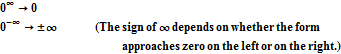
Let's start by considering why 00 is indeterminate, while 0±∞ is determinant - why is this the case? We can see that 0±∞ must tend toward 0 because multiplying some value whose magnitude is ever-shrinking by itself a greater and greater number of times, will just give us a third value whose magnitude is also decreasing indefinitely (i.e. tending toward 0).
However, if we think about 00, we can see that we run into the problem that we don't know the relationship between the base and the exponent:
It could be that the magnitude of the base decreases "much faster" than the magnitude of the exponent, in which case 00 would tend toward 0. (Hint: think about a function where the base stays fixed at zero while the exponent tends toward zero).
It could be that the magnitude of the exponent decreases "much faster" than the magnitude of the base, in which case 00 would tend toward 1. (Hint: think about a function where the base tends toward zero, but the exponent stays fixed at zero).
As in other examples, until we know more about the relationship between the exponent and the base in the expression 00, we don't know what to conclude about the limit behavior of f(x) as x→c.
A quick note about this example, for those of you who are interested: 00 is actually not undefined, because if you look around you can find some proofs that show that 00= 0. However, this isn't really relevant to our study of calculus, because even if 00 is not undefined when we are calculating something exactly, when we are finding the limit of f(x), we are not getting 00 exactly; instead we are trying to determine what the behavior is of f(x) as it tends toward 00, which is another way of asking what value a power approaches as both its base and its exponent tend toward zero (and we can't answer that question unless we know the relationship between the rate at which the base is tending toward zero and the rate at which the exponent is tending toward zero).
The Indeterminate Forms 1±∞ versus the Determinant Form a±∞
Now let's consider why 1±∞ is indeterminate, while c±∞ (for c≠1 and c>0) is determinant - why is this the case?
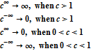
We can see that when c>1, c∞ must tend toward ∞, because multiplying some positive value greater than one by itself a greater and greater number of times will give us larger and larger values (and we can obtain a value as large as we want just by making the exponent as large as we need to do this). We can see that when 0<c<1, c∞ must tend toward 0, because multiplying some positive value less than one by itself a greater and greater number of times will give us values with smaller and smaller magnitudes (or values that are closer and closer to zero).
Related to this, we can see that when c>1, c-∞ must tend toward 0, because c-∞ is really just 1/c∞, and we already know that c∞→∞ (when c>1), and 1/∞→0. Similarly, when 0<c<1, c-∞ must tend toward ∞, because c-∞ is really just 1/c∞, and we already know that c∞→0 (when 0<c<1), and 1/0→∞ (when the denominator is positive, as it is here, because it is approaching 0 from the positive side).
However, if we think about 1±∞, we can see that we run into the problem that we don't know the relationship between the base and the exponent:
It could be that the magnitude of the base tends "much more quickly" towards 1 than the magnitude of the exponent tends toward infinity, in which case 1±∞ would tend toward 1. (Hint: think about a function where the base stays fixed at one while the exponent tends toward plus or minus infinity).
It could be that the exponent tends toward positive infinity "much more quickly" than the base tends toward 1 and that the base approaches 1 from the positive side, so that the values in the base are larger than 1: in this case, 1∞ would tend toward ∞.
It could be that the exponent tends toward positive infinity "much more quickly" than the base tends toward 1 and that the base approaches 1 from the negative side, so that the values in the base are less than 1: in this case, 1∞ would tend toward 0.
It could be that the exponent tends toward negative infinity "much more quickly" than the base tends toward 1 and that the base approaches 1 from the positive side, so that the values in the base are larger than 1: in this case, 1-∞ would tend toward 0 (because 1-∞ is really just 1/1∞, and when the base is less than 1, 1/1∞ → 1/∞ → 0).
It could be that the exponent tends toward negative infinity "much more quickly" than the base tends toward 1 and that the base approaches 1 from the negative side, so that the values in the base are less than 1: in this case, 1-∞ would tend toward ∞ (because 1-∞ is really just 1/1∞, and when the base is less than one, 1/1∞ → 1/0 → ∞). (We know that 1/0 → ∞ instead of -∞ in this case because 1∞ is approaching zero from the positive side.)
As in other examples, until we know more about the relationship between the exponent and the base in the expression 1±∞, we don't know what to conclude about the limit behavior of f(x) as x→c.
We can use similar reasoning to better understand the Indeterminate Forms ∞0 versus the Determinant Forms ∞a and ∞±∞, which is the last set of forms on our table.
To finish this lecture, let's look at a few more examples, some of which use some techniques that we have not used in the earlier example problems.
Some further examples of limit problems that can be solved algebraically:
Example 15: Using Factoring to Eliminate the Indeterminate Form 0/0
For this equation, directly substituting c into f(x) will again give us 0/0, which is undefined. However, while a/0 is undefined for all values of a, a fraction where the top remains fixed at a non-zero value and where the bottom approaches (but does not reach) zero actually approaches positive or negative infinity (depending on the signs of the numerator and denominator). To determine where f(x) may increase versus decrease without bound (i.e. whether the infinity should have a positive or negative sign in front of it), we must look at each one-sided limit separately:
Find the limit of f(x) as x approaches 0:
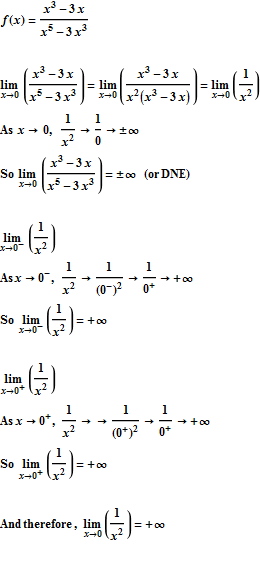
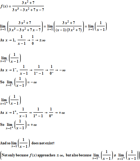
Example 16: Using factoring to eliminate the indeterminate form 0/0, with differences in the limit when we evaluate it from the left versus from the right
This function is similar to the last function; however, we notice that this time the right and left limits differ in sign/direction:
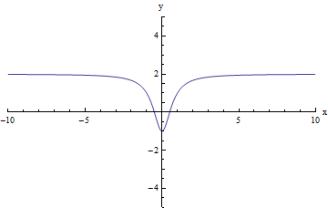
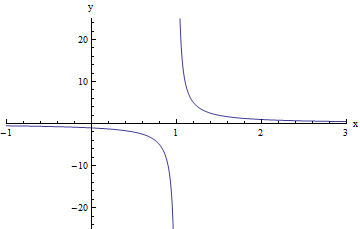
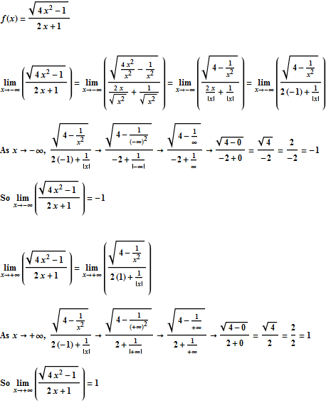
Example 17: Using division by a power of x, even when the fraction includes a radical sign, to eliminate the indeterminate form ±∞/±∞
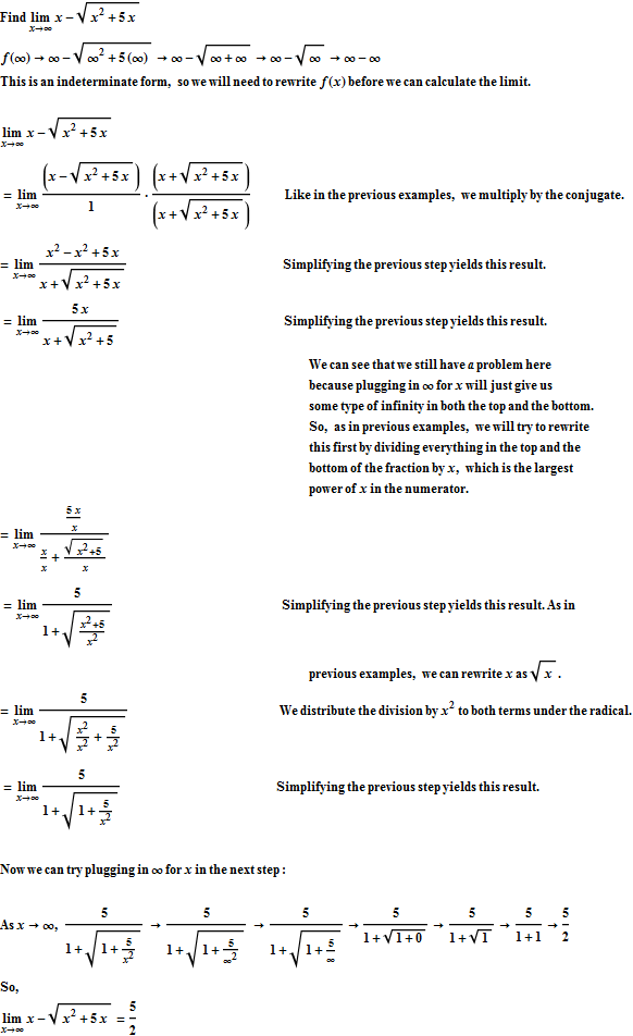
This function is similar to examples 7, 8, and 9, except that here a modified technique is necessary in order to rewrite the equation so that it can be evaluated through substitution. This time, because of the existence of the radical in the numerator, we have to divide by the square root of x2, and since this will always be positive, we must be extra careful to keep track of the signs:
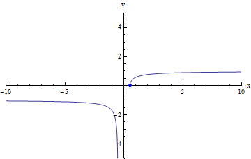
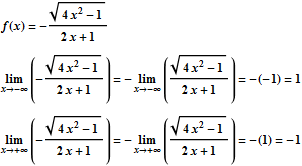
There is no reason why our limit would need to be negative as x becomes "more negative" (i.e. as x → - ∞) or that it would need to be positive as x becomes "more positive" (i.e. as x → + ∞). For example, we could have the opposite case, as we do in the function given in the following graph:
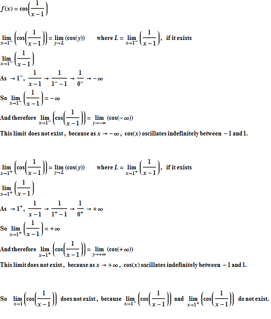
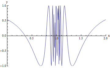
Example 18: Using substitution to evaluate a limit that can't be evaluated using one of the previous methods
And finally we have a function which has oscillating behavior around x=c, and therefore to calculate the limit here algebraically, we break the problem down into two distinct limit questions:
At this point we should be able to find all kinds of limits, either by looking at the graph of the function, or by manipulating the equation for the function algebraically!
And we should also be able to explain why some undefined values that we get when we calculate f(c) are determinant and why others are indeterminate
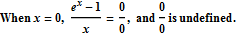

 is undefined over the set of real numbers whenever n is negative, because it will produce an imaginary number in this case. Because